PS2 Linux Programming
Introducing The 3rd Dimension
Introduction
This tutorial will introduce the background to the main techniques that are necessary in order to manipulate and view objects in three dimensions. Because of the sequential nature of 3D graphics rendering, and because there are so many calculations to be done on large volumes of data, the entire process is broken down into component steps or stages. These stages are serialised into the so called 3D graphics pipeline
In a 3D rendering system, multiple Cartesian coordinate systems (x, y, z) are used at different stages of the pipeline. Whilst being used for different purposes, each coordinate system provides a precise mathematical method of locating and representing objects in 3D space. Not surprisingly these different coordinate systems are often referred to as a 3D "space".
Objects in a 3D scene and the scene itself are sequentially converted, or transformed, through five coordinate systems when proceeding through the 3D pipeline. A brief overview of these coordinate systems is given below.
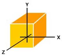
The Local Coordinate System or Model Space is where each model is defined in its own coordinate system. The origin is some point in or on the model such as at a vertex of the cube model shown in Figure 1. The cube in figure 1 used a Right Handed Coordinate system where the +x axis points to the right, the +y axis points up and the +z axis points out of the paper (or screen). There is also a Left Handed Coordinate system where the +x axis points to the right, the +y axis points up and the +z axis points in to the paper (or screen).
Figure 1
The World Coordinate System or World Space is where models are placed and orientated in the actual 3D world. Models normally undergo rotation and translation transformations when moving from their local to the world coordinate system.
The View or Camera Coordinate system (View or Camera Space) is a coordinate system defined relative to a virtual camera or eye that is located in world space. The view camera is positioned by the user or application at some point in the 3D world coordinate system. The world space coordinate system is transformed such that the camera becomes the origin of the coordinate system, with the camera looking straight down it’s z-axis into the scene. Whether z values are increasing or decreasing as an observer looks into the scene away from the camera is up to the programmer.
A view volume is created by a projection, which as the name suggests, projects the scene onto a window in front of the camera. The shape of the view volume is either rectangular (called a parallel or orthogonal projection), or a pyramidal (called a perspective projection), and this latter volume is called the view frustum. The view volume defines what the camera will see, but just as importantly it defines what the camera will not see. Many objects and parts of the world can be discarded at this stage of the pipeline thus preventing much wasted processing of objects that will not appear on the window.
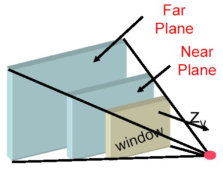
Figure 2
The frustum looks like a pyramid with its top cut off as shown in Figure 2. The top of the frustum is called the near (or front) clipping plane and the back is called the far (or back) clipping plane. The entire rendered 3D scene must fit between the near and far clipping planes, and also be bounded by the sides and top of the frustum. If triangles of the model (or parts of the world space) fall outside the frustum, they should be discarded and not be processed further. Similarly, if a triangle is partly inside and partly outside the frustum, the external portion should be clipped off at the frustum boundary and not processed further. Objects (or parts of objects) inside the view frustum will be processed further by the graphics pipeline. Although the view space frustum has clipping planes, clipping is normally performed when the frustum is transformed into clip space.
Clip Space is similar to View Space, but the frustum is now transformed into a cube shape, with the x, y and z coordinates of a scene being normalised, typically to a range between –1 and 1. This transformation greatly simplifies clipping calculations.
Screen Space is where the 3D image is converted into 2D screen coordinates for 2D display. Note that the z coordinate is still retained by the graphics systems for depth and hidden surface removal calculations. The final phase of the process is the conversion of the scene into pixels, this being called rasterisation.
In a computer game the position and orientation of objects change from frame to frame to create the illusion of movement. In a 3D world, objects can be moved or manipulated using four operations broadly referred to as transforms; these transforms will be presented below. The transforms are performed on the vertices of an object using different types of transformation matrices. All of these transform operations are affine: an affine transformation preserves parallelism of lines, though distance between points can change. These transforms are used when moving objects within a particular coordinate system or space, or when changing between spaces.
1. Translation: This is the movement or translation of an object along any of the three axes to move that object to a new location. The translation matrix is shown below where Tx, Ty and Tz are the translation components along the x, y and z axes respectively.
Rotation: This is the rotation of an object around one of it’s axes. In the simplest case, where the object to be rotated is positioned at the origin of the coordinate system, the multiplication of each vertex of the model by the rotation matrix will produces the new coordinates for that vertex. If an object is it to be rotated around more than one axis (x, y, and/or z) simultaneously, the ordering of the rotation calculations is important, as different ordering can produce different visual results. The rotation matrix for each axes is given below.
Scaling: This is the resizing of a model, which is used to shrink or expand the model. In this transform each vertex of a model is multiplied by a scaling factor, S, which will increase the size of the model by the factor S. Scaling can be uniform, where all three axes are scaled equally, or each vertex can be scaled by a different amount. Negative scale factors can produce a mirror image reflection of the object. The Scaling matrix is given below.
Shearing: Shearing (also called Skewing), changes the shape of a model by manipulating it along one or more of it’s axes. The (x,y) shear matrix is given below and there are similar matrices for the (x, z) and the (y, z) shears.
The transformation matrices given above can be combined to form a compound transformation. A combined transformation is produced by concatenating the individual transformation matrices to produce a single compound transformation matrix.
Transform processing efficiency comes from the fact that multiple matrix operations can be concatenated together into a single matrix and applied to the vertices of a model as a single matrix operation. This can spreads the matrix setup costs operation over the entire scene.
As a model travels down the graphics pipeline, it is transformed from one coordinate system to another. When performing this conversing, many of the basic transforms described above will be used. Some might be as simple as a translation or rotation, or be more complex, involving the combination of two or more concatenated transformation matrices. For example, transforming from world space to view space typically involves a translation and a rotation. The main coordinate system transformations will be presented below.
This transformation coverts a model from its own local space to world space. Typically, a model must be positioned and orientated in the 3D world which is being constructed, so the local to world transformation usually consists of the application of a rotation matrix followed by a translation matrix. The rotation matrix provided the correct orientation for the model in world space and the translation matrix moves the model to the desired position in the world.
This transform has a number of different names depending upon which text is being read. It is often called the world to screen or world to view transformation. In order to obtain a view of the 3D world that has been created, a virtual camera must be positioned in the world. The virtual camera has a position, a direction that it is pointing or looking in (sometimes called the look vector) and a direction or orientation that is up (often called the up vector). A third vector, mutually perpendicular to both the look and the up vector is used and this is often called the Right vector. The relationship between these vectors is illustrated in figure 3.
Figure 3
Before a view of the 3d world can be obtained, all of the vertices of all of the objects in the world must be converted to camera space. This normally entails the combination of a translation followed by a rotation which converts or transforms all of the vertices in the world so that they are now positioned relative to the location and orientation of the virtual camera.
There are several methods of constructing the world to camera transformation matrix. One approach involves creating the composite view matrix directly. This uses the camera's world space position (P) and a look-at point (LA) in the scene to derive look (L), up (U) and right (R) vectors that describe the orientation of the camera space coordinate axes. The camera position is subtracted from the look-at point to produce a vector for the camera's direction vector.
![]()
Then the cross product between the look vector and the world up vector (WU) (which is normally (0, 1, 0)) is taken and normalised to produce a right vector, R.
![]()
Next, the cross product between the vectors L and R is taken to determine an up vector for the camera (vector U).
![]()
The right (R), up (U), and look (L) direction vectors describe the orientation of the coordinate axes for camera space in terms of world space.
Before rotating any of the points in the virtual world, they must all be translated so that the camera becomes the origin of our coordinate system. If the cameral is located at position (Px, Py, Pz) in the world, then all of the vertices in world coordinates must undergo a translation of (-Px, -Py, -Pz) to be described relative to the camera position. This translation can be described by the following matrix.
The points in the world must now undergo a rotation to orientate them with the camera. The camera rotation matrix can be constructed from the look, up and right vectors that have already been derived. One point to note about the camera rotation matrix is that it is constructed as an “inverse” rotation matrix (or a transposed matrix since we are dealing with an orthogonal matrix). To help visualise why this is the case, if you consider turning your head to the right, all object in view move to the left. This is same for the other two directions. The rotation matrix for the camera is thus:
The final camera matrix is obtained from concatenating the translation and rotation parts. It is important to get the order of concatenation correct: the translation is done first, followed by the rotation.
The camera matrix is therefore:
In this matrix, R, U, and L are the right, up, and view direction vectors, and P is the camera position vector in world space. This matrix contains all the elements needed to translate and rotate vertices from world space to camera space. After creating this matrix, it is a simple matter to apply additional rotation transformation matrices to the camera matrix to allow, for example, the camera to roll around it’s z or look axis.
In this tutorial the main techniques necessary in order to manipulate and view objects in three dimensions have been introduced. It has been shown how to define objects relative to a virtual camera which is located in world space. In the next tutorial, 3D viewing will be discussed where the 3D scene is projected onto a 2D screen. Hidden surface removal and clipping will also be introduced
Dr Henry S Fortuna
University of Abertay Dundee